How to shuffle ties after a sort?

When sorting a large table according to a specific metric (let’s say gene expression value), it is frequent to have ties for certain values (for example, 0 expression values). In most version of sorting, the order of the ties is preserved by the sorting. For example, with the base function order:

suppressPackageStartupMessages(library(tidyverse))

gene_exp <- tibble(
    gene_name = paste0("ENSG0", 1:9),
    exp = c(rbind(rnorm(4, mean = 2), c(0, 0, 0, 0)), 0)
)

gene_exp
## # A tibble: 9 × 2
##   gene_name   exp
##   <chr>     <dbl>
## 1 ENSG01     3.08
## 2 ENSG02     0   
## 3 ENSG03     2.21
## 4 ENSG04     0   
## 5 ENSG05     2.20
## 6 ENSG06     0   
## 7 ENSG07     2.29
## 8 ENSG08     0   
## 9 ENSG09     0
gene_exp[order(gene_exp$exp, decreasing = TRUE), ]
## # A tibble: 9 × 2
##   gene_name   exp
##   <chr>     <dbl>
## 1 ENSG01     3.08
## 2 ENSG07     2.29
## 3 ENSG03     2.21
## 4 ENSG05     2.20
## 5 ENSG02     0   
## 6 ENSG04     0   
## 7 ENSG06     0   
## 8 ENSG08     0   
## 9 ENSG09     0

Or with dplyr::arrange:

gene_exp %>%
    arrange(desc(exp))
## # A tibble: 9 × 2
##   gene_name   exp
##   <chr>     <dbl>
## 1 ENSG01     3.08
## 2 ENSG07     2.29
## 3 ENSG03     2.21
## 4 ENSG05     2.20
## 5 ENSG02     0   
## 6 ENSG04     0   
## 7 ENSG06     0   
## 8 ENSG08     0   
## 9 ENSG09     0

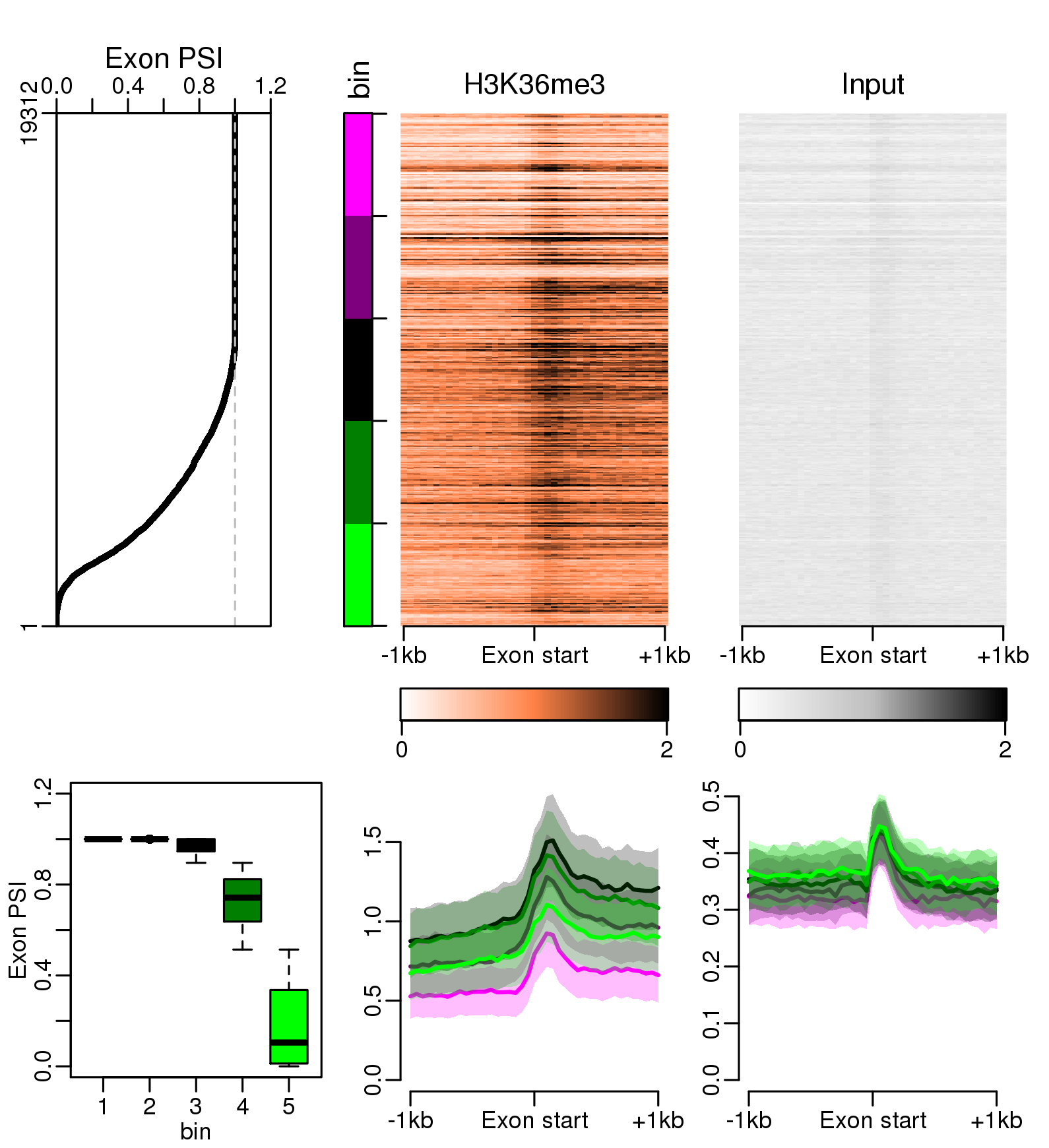
This can lead to ungraceful artefacts in some plots. For example, in the plot bellow we look at a certain epigenetic mark (H3K36me3) at middle exons (neither first nor last exons) according to the exon inclusion ratio metric (or \(\psi\)):

Here, many exons have \(\psi = 1\), and their order default to a genomic coordinate ordering. We can see some dark horizontal stripes, that may reflect contiguous chromatin domains but distract us from the main point(s).

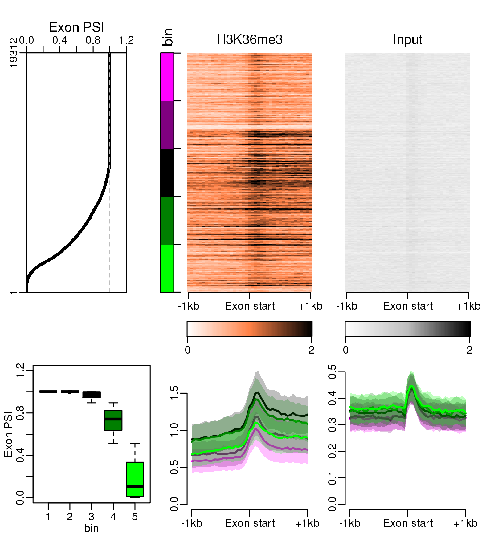
It might be better to shuffle the rows of our table that correspond to ties after our sorting.

Thinking about how to do it, the first approach that came to my mind was a split - apply - combine, where we first split the data frame, apply a shuffling if needed, and combine it back. With our toy example:

gene_exp %>%
    group_by(exp) %>%
    sample_frac(size = 1, replace = FALSE) %>% # shuffeling within each group
    ungroup() %>%
    arrange(desc(exp))
## # A tibble: 9 × 2
##   gene_name   exp
##   <chr>     <dbl>
## 1 ENSG01     3.08
## 2 ENSG07     2.29
## 3 ENSG03     2.21
## 4 ENSG05     2.20
## 5 ENSG02     0   
## 6 ENSG06     0   
## 7 ENSG04     0   
## 8 ENSG08     0   
## 9 ENSG09     0

Here our ties are correctly shuffled. \o/

Actually, never mind, the grouping is totally unnecessary, one can simply shuffle the dataset first, and sort it later:

gene_exp %>%
    sample_frac(size = 1, replace = FALSE) %>% # shuffeling within each group
    arrange(desc(exp))
## # A tibble: 9 × 2
##   gene_name   exp
##   <chr>     <dbl>
## 1 ENSG01     3.08
## 2 ENSG07     2.29
## 3 ENSG03     2.21
## 4 ENSG05     2.20
## 5 ENSG04     0   
## 6 ENSG02     0   
## 7 ENSG08     0   
## 8 ENSG06     0   
## 9 ENSG09     0

A second approach could be to generate a column of random value and use it to breaks the ties in the sort:

gene_exp %>%
    mutate(rand = runif(nrow(gene_exp))) %>%
    arrange(desc(exp), rand) %>%
    select(-rand)
## # A tibble: 9 × 2
##   gene_name   exp
##   <chr>     <dbl>
## 1 ENSG01     3.08
## 2 ENSG07     2.29
## 3 ENSG03     2.21
## 4 ENSG05     2.20
## 5 ENSG08     0   
## 6 ENSG04     0   
## 7 ENSG06     0   
## 8 ENSG02     0   
## 9 ENSG09     0

It’s working too! \o/

There is even no need to create the new column at all:

gene_exp %>%
    arrange(desc(exp), runif(nrow(gene_exp)))
## # A tibble: 9 × 2
##   gene_name   exp
##   <chr>     <dbl>
## 1 ENSG01     3.08
## 2 ENSG07     2.29
## 3 ENSG03     2.21
## 4 ENSG05     2.20
## 5 ENSG04     0   
## 6 ENSG02     0   
## 7 ENSG06     0   
## 8 ENSG08     0   
## 9 ENSG09     0

Since we now have two approaches, a benchmark is needed to compare them speed-wise. We will do it on a larger dataset to be a bit more realistic:

gene_exp <- tibble(
    gene_name = paste0("ENSG0", 1:10000),
    exp = c(rbind(rnorm(5000, mean = 2), rep(0, 5000)))
)

gene_exp
## # A tibble: 10,000 × 2
##    gene_name   exp
##    <chr>     <dbl>
##  1 ENSG01    3.71 
##  2 ENSG02    0    
##  3 ENSG03    1.75 
##  4 ENSG04    0    
##  5 ENSG05    2.96 
##  6 ENSG06    0    
##  7 ENSG07    0.723
##  8 ENSG08    0    
##  9 ENSG09    2.57 
## 10 ENSG010   0    
## # … with 9,990 more rows
library(microbenchmark)

microbenchmark(

    "shuffle_sort" = gene_exp %>%
        sample_frac(size = 1, replace = FALSE) %>%
        arrange(desc(exp)),

    "random_column_unif" = gene_exp %>%
        arrange(desc(exp), runif(nrow(gene_exp))),

    "random_column_norm" = gene_exp %>%
        arrange(desc(exp), rnorm(nrow(gene_exp)))

) %>% autoplot() +
    theme_bw(base_size = 16)
## Coordinate system already present. Adding new coordinate system, which will replace the existing one.

And now I have stacked profiles of epigenetic marks that smooth-out unwanted irregularities, by shuffling the ties: