The shape of DNA
Graphical abstract:
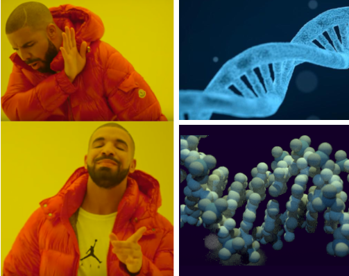
Molecular biologists and biochemists are quite sensitive on the topic of DNA representation. Many of them will be triggered when the looping of the DNA is misrepresented as a left-handed helix instead of a right-handed one (what we mean by that is that when one looks at DNA from ‘within’ the helix, they turn clock-wise as they get more distant). I am not quite offended by this mistake, as I hardly remember if (B-)DNA is right-handed or left-handed, and what right-handed and left-handed means in the context of an helix.
I am paying more attention to the fact that the DNA double-helix has two grooves of unequal size, one big major groove, and a narrow minor groove. It matters because transcription factors can bind either to the major groove or to the minor groove, and the rules governing their sequence specificity won’t be the same in each case.
I sometimes do complain about that:
Should someone tell them about the whole major/minor groove thing? https://t.co/KPq9iFkUge
— Guillaume Devailly (@G_Devailly) December 13, 2018
As others do:
GREAT! But <pedant=ON> NO MAJOR/MINOR GROOVE!!! See example below from @PDBeurope </pedant=OFF> :-) ;-)https://t.co/1rX87naLgg
— Geoff Barton 🇪🇺 (@gjbarton) December 13, 2018
And guess what, complaining on twitter can sometime have an impact!
The great christmas elves in the @emblebi comms department have created your handy, right handed (right) from left handed (wrong), minor groove containing card for genomics comms professionals. (Even more Hi res media available on demand...) pic.twitter.com/mQpZHvqDO6
— Ewan Birney (@ewanbirney) December 14, 2018
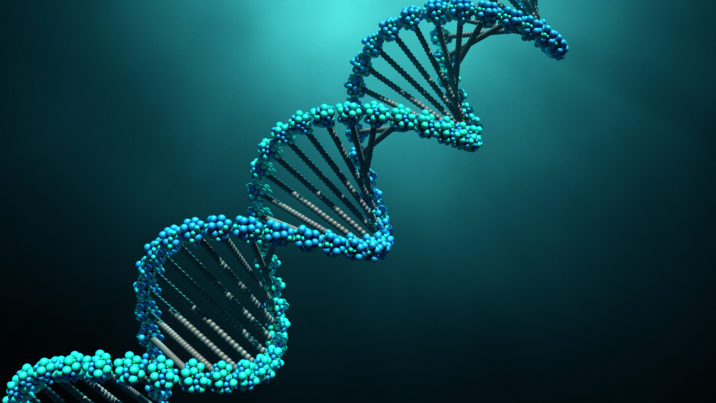
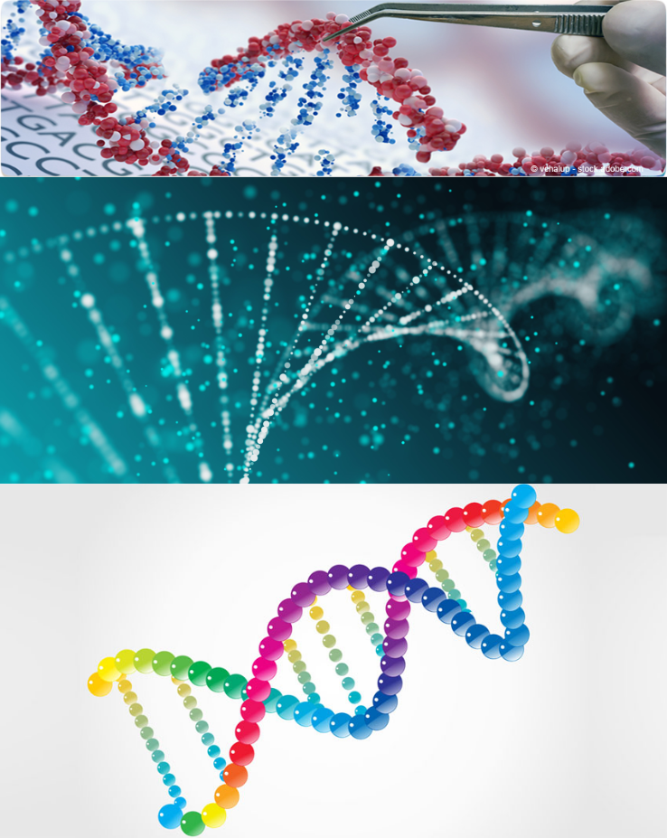
My other pet peeve is when artistic views of DNA show unnecessary “asperities” in the texture of DNA to “make it more real” while still representing a very basic rope-ladder shape.
For examples:
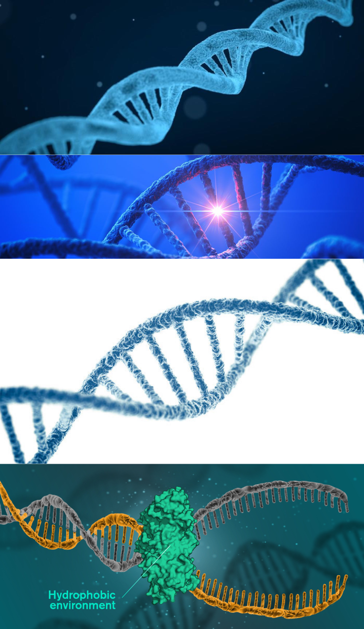
These visualisations are so popular that any efforts to name and shame will results in either naming the entire universe or hand picking some for biased reasons. I’ll hand pick one nonetheless: the homepage of Genome Biology. 😑

It seems that at some point, some artists began to realise that the DNA rope-ladder was actually made of atoms. They decided to represent atoms as spheres, which make sense. But instead of positioning the spheres on realistic positions, or by simply downloading available 3D models, they did that:
🤦
And the endless list of bad DNA visualisation goes on.
I find those view annoying, because we have known the exact structure of the B DNA helix for a long time, with many 3D models freely available! One could take those, apply a bumpy fluorescent blue texture in front of a black background and produce similarly impressive artistic views that would be much closer to the reality.
Let me try to be clearer:
-
my rant is not against the rope and ladder view of DNA. It is a useful representation, but for diagram and such.
-
it is not against artistic views, they are both useful and often spectacular when well done.
-
it is about one bad type of artistic view that is representing DNA as a “rope ladder” while adding asperities to make it more realistic, ignoring that the atomic structures of DNA had been known since before I was born.
Thankfully, the brilliant PDB’s molecule of the month team offers us some hope. Let’s all admire the DNA molecule:
But enough complaining for today, let’s try to be a bit more constructive and build our own scientifically accurate artistic view of DNA with R!
First we download and parse the PDB structure 1BNA, which is a structure file of a 12 nucleotide long DNA double helix in B shape. Let’s use the CRAN package bio3d:
library(bio3d)

dna <- read.pdb("1BNA")
##   Note: Accessing on-line PDB file
head(dna$atom)
##   type eleno elety  alt resid chain resno insert      x      y      z o     b
## 1 ATOM     1   O5' <NA>    DC     A     1   <NA> 18.935 34.195 25.617 1 64.35
## 2 ATOM     2   C5' <NA>    DC     A     1   <NA> 19.130 33.921 24.219 1 44.69
## 3 ATOM     3   C4' <NA>    DC     A     1   <NA> 19.961 32.668 24.100 1 31.28
## 4 ATOM     4   O4' <NA>    DC     A     1   <NA> 19.360 31.583 24.852 1 37.45
## 5 ATOM     5   C3' <NA>    DC     A     1   <NA> 20.172 32.122 22.694 1 46.72
## 6 ATOM     6   O3' <NA>    DC     A     1   <NA> 21.350 31.325 22.681 1 48.89
##   segid elesy charge
## 1  <NA>     O   <NA>
## 2  <NA>     C   <NA>
## 3  <NA>     C   <NA>
## 4  <NA>     O   <NA>
## 5  <NA>     C   <NA>
## 6  <NA>     O   <NA>
We keep only the lines and columns that we will use, notably getting rid of a few water molecules.
library(dplyr)
##
## Attachement du package : 'dplyr'
## Les objets suivants sont masqués depuis 'package:stats':
##
##     filter, lag
## Les objets suivants sont masqués depuis 'package:base':
##
##     intersect, setdiff, setequal, union
dnamod <- filter(dna$atom, type == "ATOM" ) %>%
    select(x, y, z, atom = "elesy")

head(dnamod)
##        x      y      z atom
## 1 18.935 34.195 25.617    O
## 2 19.130 33.921 24.219    C
## 3 19.961 32.668 24.100    C
## 4 19.360 31.583 24.852    O
## 5 20.172 32.122 22.694    C
## 6 21.350 31.325 22.681    O
We use the rayrender package to hand-craft our scientifically accurate artistic view of a DNA molecule. It is a quite new ray-tracing tool, not particularly designed to render macro-molecules. This means that we have to do some dirty work ourselves.
First we centre the molecule coordinates, to be able to point the virtual camera to the centre of the DNA molecule by simply targeting the XYZ point: c(0, 0, 0).
summarise_if(dnamod, is.numeric, min)
##       x     y       z
## 1 4.025 8.032 -11.401
summarise_if(dnamod, is.numeric, max)
##        x      y      z
## 1 26.506 34.195 31.084
dnamod <- mutate(dnamod, x = x - mean(x), y = y - mean(y), z = z - mean(z))

summarise_if(dnamod, is.numeric, min)
##           x         y        z
## 1 -10.69357 -12.94741 -20.2247
summarise_if(dnamod, is.numeric, max)
##          x        y       z
## 1 11.78743 13.21559 22.2603
We create a look-up table containing some details about each atom in the molecule. We use some standard, non-artistic, colours first:
unique(dnamod$atom)
## [1] "O" "C" "N" "P"
elref <- tribble(
    ~atom, ~atomic_mass, ~color,
    "C", 12, "lightgrey",
    "N", 14, "darkblue",
    "O", 16, "darkred",
    "P", 31, "darkorange"
)
Now let’s build our model. Rayrender’s function sphere() is not vectorised.
Therefore we call sphere() one time per atom, using purrr::map_dfr() to be fancy:
library(rayrender)
library(purrr)

mol <-  map_dfr(
    unique(dnamod$atom), # one iteration for each tom type, C, N, O, P
    function(ato) {
        melref = filter(elref, atom == ato)
        dnamo = filter(dnamod, atom == ato)
        map_dfr(seq_len(nrow(dnamo)), function(i) { # one iteration per atom
            sphere(
                x = dnamo$x[i], y = dnamo$y[i], z = dnamo$z[i],
                radius = 0.4 * melref$atomic_mass^(1/3),
                # radius is proportionnal to the cubic root of the atomic mass.
                # 0.4 is a magic number leading to a visualisation that doesn't look too bad.
                material = diffuse(color = melref$color)
            )
        })
    }
)
We now render our first scene. Rayrender is basically ray-tracing on CPU, which means it is quite slow. So it’s best to render small scenes first to find the appropriate parameters, before rendering a beautiful one once you are happy with the scene.
A scene is composed of objects (here described in the mol tibble), and a camera that has a location, and point to something.
We centred our object, so we tell the camera to point at c(0, 0, 0). It’s probably best if the camera is somewhere outside of the object. I played a bit with the lookfrom parameter, and found the values c(60, 0, -10) reasonably satisfying. So behold the following rendering:
render_scene(
    mol,
    lookfrom = c(60, 0, -10),
    lookat = c(0, 0, 0),
    parallel = TRUE, width = 800, height = 500, samples = 100,
    backgroundhigh = "white", backgroundlow = "white"
)
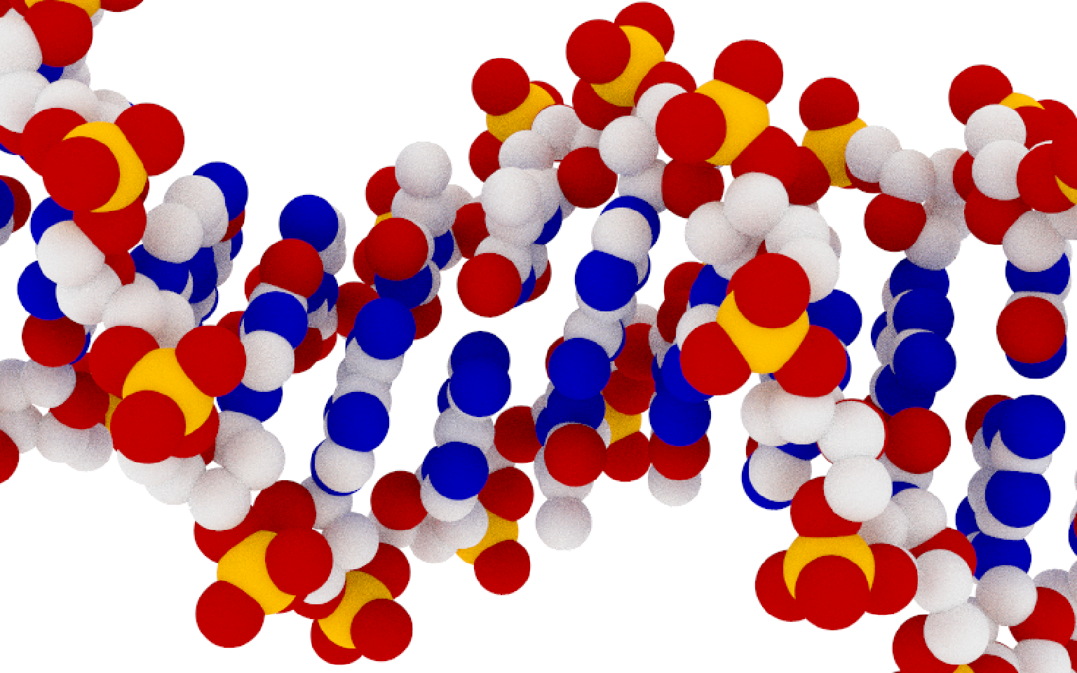
Figure 1: Scientifically accurate, non artistic view of DNA.
Now let’s try to render this non-artistic, a bit boring, view of DNA into an artistic one. I’m no artist, but let’s put a darker background, two light sources of different colours, and an invisible metallic mirror in the background to generate some dirty reflections to make the scene less empty. Let’s also pick fairly neutral colours for the atoms, and fiddle with the camera aperture and focal distance.
elref <- tribble(
    ~atom, ~atomic_mass, ~color,
    "C", 12, "azure1",
    "N", 14, "azure3",
    "O", 16, "azure4",
    "P", 31, "steelblue4"
)

mol <-  map_dfr(
    unique(dnamod$atom),
    function(ato) {
        melref = filter(elref, atom == ato)
        dnamo = filter(dnamod, atom == ato)
        map_dfr(seq_len(nrow(dnamo)), function(i) { # one iteration per atom
            sphere(
                x = dnamo$x[i], y = dnamo$y[i], z = dnamo$z[i],
                radius = 0.4 * (melref$atomic_mass)^(1/3),
                material = diffuse(color = melref$color)
            )
        })
    }
) %>%
    # first light, magic numbers
    add_object(sphere(
        x = 120, y = 50, z = -10, material = light("dodgerblue", intensity = 3000)
    )) %>%
    # second light, magic numbers
    add_object(sphere(
        x = 20, y = 70, z = -10, material = light("darkolivegreen1", intensity = 3000)
    )) %>%
    # a big spheric mirror somewhere on the back
    add_object(sphere(
        x = -450, y = -100, z = 160, radius = 400, material = metal(fuzz = 0.05)
    ))

render_scene(
    mol,
    lookfrom = c(60, 0, -10),
    lookat = c(0, 0, 0),
    aperture=0.8, focal_distance = 55,  clamp_value = 5,
    ambient_light = TRUE, backgroundhigh = "#010005", backgroundlow = "black",
    parallel = TRUE, width = 800, height = 500, samples = 600
)
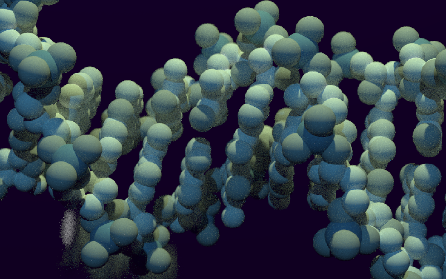
Figure 2: Scientifically accurate, totally artistic view of DNA.
Not bad! My main regret is that the PDB DNA structure 1BNA is only 12 nucleotide long. A longer DNA model might be more suitable for artistic representations, but I was too lazy to search for one or build one myself (too bad for you, 16-nucleotide long structure 3BSE).
To conclude, I’ll offer a stay-at-home challenge: try to render your own scientifically accurate artistic view of the DNA molecule, for example by changing a few parameters from this post' script. Then post it on twitter mentioning me (G_Devailly), the winner will be retweeted! 🎉
Thanks to schneu for kindly providing some proofreading.
R session details:
sessionInfo()
## R version 4.1.1 (2021-08-10)
## Platform: x86_64-pc-linux-gnu (64-bit)
## Running under: Ubuntu 20.04.3 LTS
##
## Matrix products: default
## BLAS:   /usr/lib/x86_64-linux-gnu/blas/libblas.so.3.9.0
## LAPACK: /usr/lib/x86_64-linux-gnu/lapack/liblapack.so.3.9.0
##
## locale:
##  [1] LC_CTYPE=fr_FR.UTF-8       LC_NUMERIC=C
##  [3] LC_TIME=fr_FR.UTF-8        LC_COLLATE=fr_FR.UTF-8
##  [5] LC_MONETARY=fr_FR.UTF-8    LC_MESSAGES=fr_FR.UTF-8
##  [7] LC_PAPER=fr_FR.UTF-8       LC_NAME=C
##  [9] LC_ADDRESS=C               LC_TELEPHONE=C
## [11] LC_MEASUREMENT=fr_FR.UTF-8 LC_IDENTIFICATION=C
##
## attached base packages:
## [1] stats     graphics  grDevices utils     datasets  methods   base
##
## other attached packages:
## [1] purrr_0.3.4      rayrender_0.21.2 dplyr_1.0.7      bio3d_2.4-2
##
## loaded via a namespace (and not attached):
##  [1] Rcpp_1.0.7       highr_0.9        bslib_0.3.0      compiler_4.1.1
##  [5] pillar_1.6.2     jquerylib_0.1.4  tools_4.1.1      digest_0.6.27
##  [9] lattice_0.20-45  lubridate_1.7.10 jsonlite_1.7.2   evaluate_0.14
## [13] lifecycle_1.0.0  tibble_3.1.4     pkgconfig_2.0.3  rlang_0.4.11
## [17] DBI_1.1.1        yaml_2.2.1       parallel_4.1.1   blogdown_1.5
## [21] xfun_0.26        emo_0.0.0.9000   fastmap_1.1.0    raster_3.4-13
## [25] stringr_1.4.0    knitr_1.34       generics_0.1.0   sass_0.4.0
## [29] vctrs_0.3.8      tidyselect_1.1.1 grid_4.1.1       glue_1.4.2
## [33] R6_2.5.1         fansi_0.5.0      rmarkdown_2.11   bookdown_0.22
## [37] sp_1.4-5         magrittr_2.0.1   codetools_0.2-18 htmltools_0.5.2
## [41] ellipsis_0.3.2   assertthat_0.2.1 rayimage_0.6.2   utf8_1.2.2
## [45] stringi_1.7.4    crayon_1.4.1
Guillaume Devailly
Researcher in farm animal epigenetics
Researcher in farm animal epigenetics at INRAE, France.