Foreword

We recently developed an R package, named {epistack}, to visualise epigenomic data. Epistack is available on github and Bioconductor.

The best place to learn more about it is probably the package’s vignette.

The following is a silly attempt at benchmarking {epistack} againts the great {EnrichedHeatmap}.

TLDR: both are fast enough.

---

Generating benchmark datasets

To compare {epistack} with other methods, we will use an artificially generated dataset. We will generate artificial datasets of various regon length using a function defined bellow (there is no need to understand how this function works, it’s simply generate a dumy object that can be input to plotEpistack()).

library(GenomicRanges)
library(epistack)

epidataset <- function(n) {
  # fist we generate a fake epigenetic signal matrix
  mat = matrix(nrow = n, ncol = 50)
  for(i in seq_len(nrow(mat))) {
    mat[i, ] = runif(50) +
      c(sort(abs(rnorm(50)))[1:25], rev(sort(abs(rnorm(50)))[1:25]))*i/(n/4)
  }
  
  # we then embeded the matrix in a GRanges object
  testdat <- GRanges(
    rep("chr1", n),
    IRanges(rep(1, n), rep(2, n)),
    mcols = mat
  )
  testdat$expr <- exp(seq(from = 0, to = 3, length.out = n)) 
  testdat <- testdat[seq(length(testdat), 1),]
  testdat <- addBins(testdat, nbins = 5)
  testdat
}

The function is working as intended:

epidataset(100)[, 49:52]
#> GRanges object with 100 ranges and 4 metadata columns:
#>         seqnames    ranges strand | mcols.V49 mcols.V50      expr       bin
#>            <Rle> <IRanges>  <Rle> | <numeric> <numeric> <numeric> <numeric>
#>     [1]     chr1       1-2      * |  0.952068  0.179671   20.0855         1
#>     [2]     chr1       1-2      * |  0.478568  0.340969   19.4860         1
#>     [3]     chr1       1-2      * |  0.412846  0.497083   18.9044         1
#>     [4]     chr1       1-2      * |  0.684431  0.437699   18.3401         1
#>     [5]     chr1       1-2      * |  0.580179  0.901338   17.7927         1
#>     ...      ...       ...    ... .       ...       ...       ...       ...
#>    [96]     chr1       1-2      * | 0.0516165 0.7985905   1.12886         5
#>    [97]     chr1       1-2      * | 0.2357467 0.3174062   1.09517         5
#>    [98]     chr1       1-2      * | 0.6359180 0.2045663   1.06248         5
#>    [99]     chr1       1-2      * | 0.6136850 0.0915456   1.03077         5
#>   [100]     chr1       1-2      * | 0.0981223 0.7333909   1.00000         5
#>   -------
#>   seqinfo: 1 sequence from an unspecified genome; no seqlengths
epidataset(10000)[, 49:52]
#> GRanges object with 10000 ranges and 4 metadata columns:
#>           seqnames    ranges strand | mcols.V49 mcols.V50      expr       bin
#>              <Rle> <IRanges>  <Rle> | <numeric> <numeric> <numeric> <numeric>
#>       [1]     chr1       1-2      * |  0.890472  0.695199   20.0855         1
#>       [2]     chr1       1-2      * |  0.744390  0.424815   20.0795         1
#>       [3]     chr1       1-2      * |  0.443652  0.298934   20.0735         1
#>       [4]     chr1       1-2      * |  0.954323  0.983730   20.0675         1
#>       [5]     chr1       1-2      * |  0.307858  0.894837   20.0614         1
#>       ...      ...       ...    ... .       ...       ...       ...       ...
#>    [9996]     chr1       1-2      * |  0.342960 0.6116082    1.0012         5
#>    [9997]     chr1       1-2      * |  0.389621 0.0192827    1.0009         5
#>    [9998]     chr1       1-2      * |  0.499694 0.0725932    1.0006         5
#>    [9999]     chr1       1-2      * |  0.886972 0.9410834    1.0003         5
#>   [10000]     chr1       1-2      * |  0.243264 0.0821325    1.0000         5
#>   -------
#>   seqinfo: 1 sequence from an unspecified genome; no seqlengths

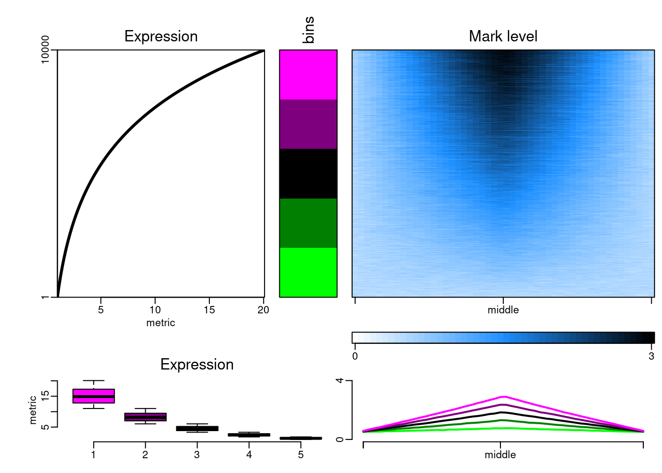
The datasets can then be plotted with epistack:

plotEpistack(
  epidataset(10000), 
  zlim = c(0, 3), ylim = c(0, 4), tints = "dodgerblue",
  patterns = "mcols", titles = "Mark level", x_labels = c("", "middle", ""), 
  metric_col = "expr", metric_title = "Expression"
)

We can now generate a benchmark dataset containing GRanges objects of various lengths.

sizes <- c(
  1000, 2000, 5000,
  10000, 20000, 50000,
  100000, 200000
)

benchdata <- lapply(sizes, epidataset)

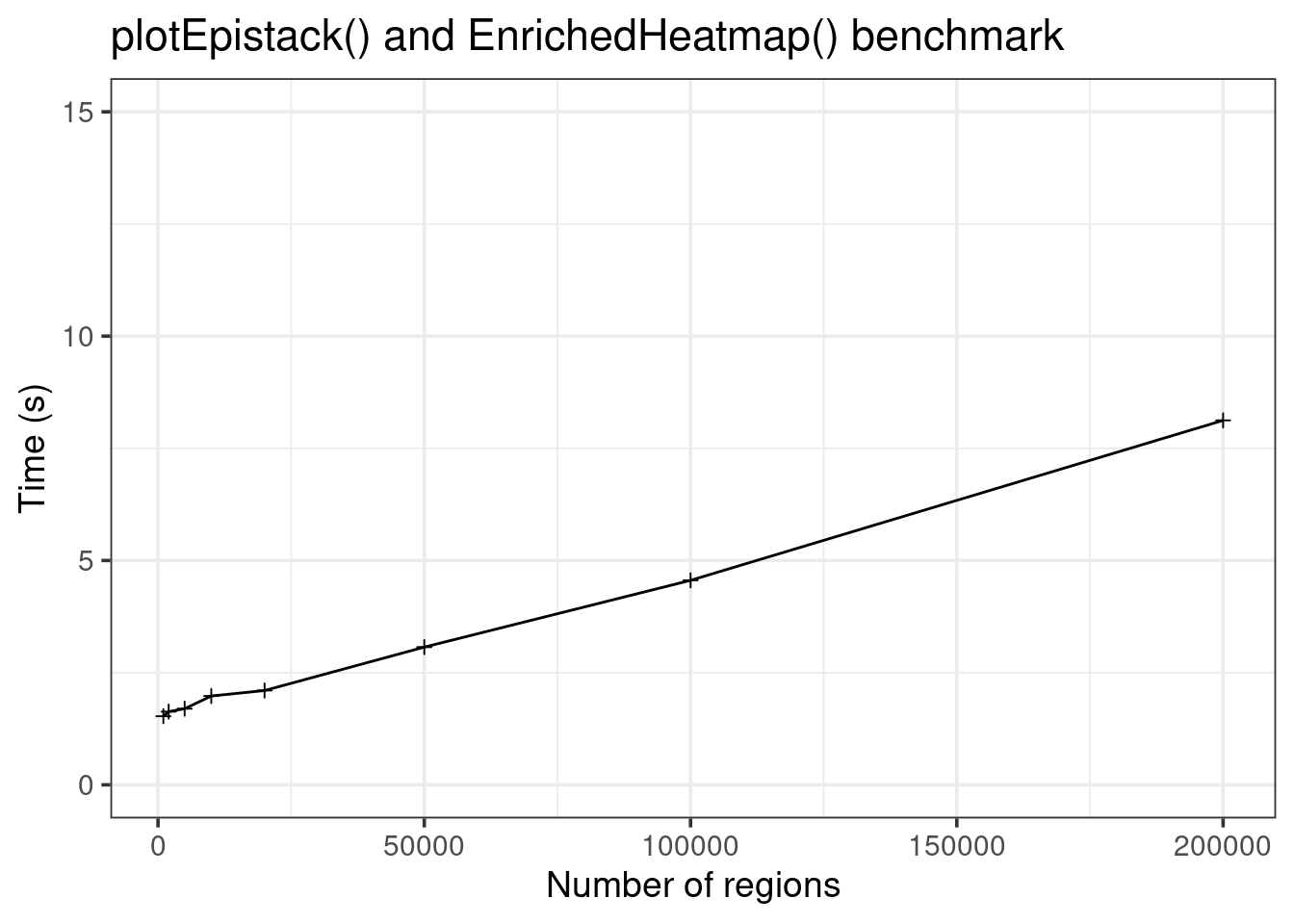
Benchmarking epistack()

runtimes <- sapply(benchdata, function(x) system.time(
  plotEpistack(
    x, 
    zlim = c(0, 3), ylim = c(0, 4), tints = "dodgerblue",
    patterns = "mcols", titles = "Mark level", x_labels = c("", "middle", ""), 
    metric_col = "expr", metric_title = "Expression"
  )
)["elapsed"])

runtimes2 <- sapply(benchdata, function(x) system.time(
  plotEpistack(
    x, 
    zlim = c(0, 3), ylim = c(0, 4), tints = "dodgerblue",
    patterns = "mcols", titles = "Mark level", x_labels = c("", "middle", ""), 
    metric_col = "expr", metric_title = "Expression"
  )
)["elapsed"])

library(ggplot2)

data.frame(size = sizes, time = runtimes) |>
  ggplot(aes(x = size, y = time)) +
    geom_line() +
    geom_point(shape = 3) +
    theme_bw(base_size = 14) +
    labs(x = "Number of regions", y = "Time (s)",
         title = "plotEpistack() and EnrichedHeatmap() benchmark") +
    coord_cartesian(ylim = c(0, 15))

Comparison with EnrichedHeatmap

First we transform the benchmark dataset into the format needed by {EnrichedHeatmap}:

library(EnrichedHeatmap)
# we first make a dummy normalizedMatrix object to later steal its attributes
load(
  system.file("extdata", "chr21_test_data.RData", package = "EnrichedHeatmap")
)
ehmat <- normalizeToMatrix(
  meth, 
  resize(cgi, width = 1, fix = "center"),
  value_column = "meth", mean_mode = "absolute",
  extend = 2500, w = 100, smooth = TRUE
)

# we then apply the attributes to the signal matrices in benchdata
ehbenchdata <- lapply(
  benchdata,
  function(x) {
    mat <- as.matrix(mcols(x)[, 1:50])
    mdim <- dim(mat)
    mdimnames <- dimnames(mat)
    mostattributes(mat) <- attributes(ehmat)
    dim(mat) <- mdim
    dimnames(mat) <- mdimnames
    mat
  }
)

We can now call EnrichedHeatmap:

col_fun = circlize::colorRamp2(c(0, 1.5, 3), c("white", "dodgerblue", "black"))
EnrichedHeatmap(
    ehbenchdata[[1]], col = col_fun,
    name= "Mark level",  column_title = "Mark level")

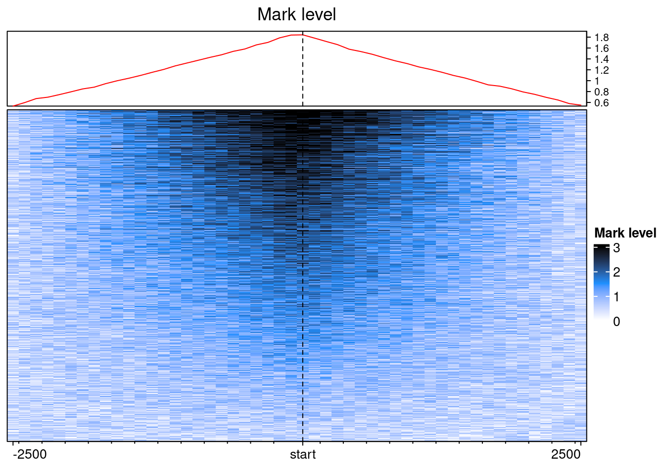
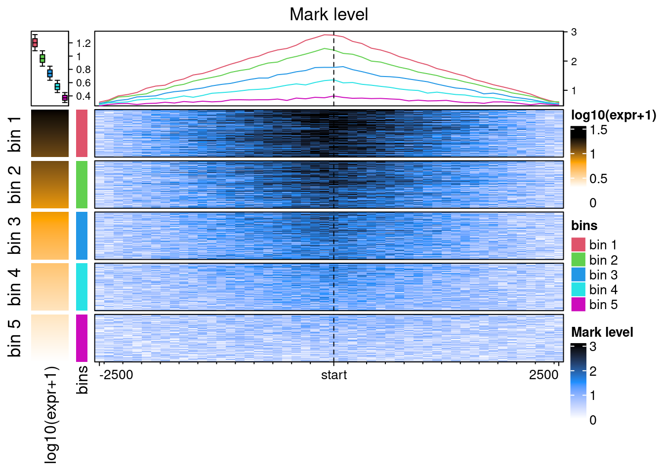
With some fiddeling, it is possible to make EnrichedHeatmap outputs equivalent to the plotEpistack’s outputs.

ht_list <- Heatmap(
  log10(benchdata[[1]]$expr+1), 
  col = c("white", "orange", "black"), name = "log10(expr+1)", 
  show_row_names = FALSE, width = unit(10, "mm"),
  top_annotation = HeatmapAnnotation(
    summary = anno_summary(
      gp = gpar(fill = 2:6),
      outline = FALSE, axis_param = list(side = "right")
    )
  )
) +
  Heatmap(
    paste("bin", benchdata[[1]]$bin),
    col = structure(2:6, names = paste("bin", 1:5)), 
    name = "bins",
    show_row_names = FALSE, width = unit(3, "mm")
  ) + 
  EnrichedHeatmap(
    ehbenchdata[[1]], col = col_fun,
    name= "Mark level",  column_title = "Mark level",
    top_annotation = HeatmapAnnotation(
      lines = anno_enriched(gp = gpar(col = 2:6))
    )
  )

draw(
  ht_list,
  split = paste("bin", benchdata[[1]]$bin), cluster_rows = FALSE
)

We can now run a benchmark. Note that there is currently a bug in EnrichedHeatmap preventing us to generate the Heatmaps with more than 100.000 regions unless we shut off rasterization.

runtimes2 <- sapply(1:8, function(i) system.time({
  
  ht_list <- Heatmap(
    log10(benchdata[[i]]$expr+1), 
    col = c("white", "orange", "black"), name = "log10(expr+1)", 
    show_row_names = FALSE, width = unit(10, "mm"),
    top_annotation = HeatmapAnnotation(
      summary = anno_summary(
        gp = gpar(fill = 2:6),
        outline = FALSE, axis_param = list(side = "right")
      )
    )
  ) +
    Heatmap(
      paste("bin", benchdata[[i]]$bin),
      col = structure(2:6, names = paste("bin", 1:5)), 
      name = "bins",
      show_row_names = FALSE, width = unit(3, "mm")
    ) + 
    EnrichedHeatmap(
      ehbenchdata[[i]], col = col_fun,
      name= "Mark level",  column_title = "Mark level",
      top_annotation = HeatmapAnnotation(
        lines = anno_enriched(gp = gpar(col = 2:6))
      )
    )
  
  draw(
    ht_list,
    split = paste("bin", benchdata[[i]]$bin), cluster_rows = FALSE,
    use_raster = FALSE
  )
  
})["elapsed"])


data.frame(
  size = c(sizes, sizes),
  time = c(runtimes, runtimes2),
  method = c(rep("epistack", 8), rep("EnrichedHeatmap", 8))) |>
  ggplot(aes(x = size, y = time, color = method)) +
    geom_line() +
    geom_point(shape = 3) +
    theme_bw(base_size = 14) +
    labs(x = "Number of regions", y = "Time (s)",
         title = "plotEpistack() benchmark") +
    coord_cartesian(ylim = c(0, 60))

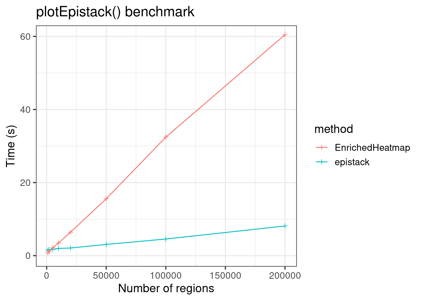
EnrichedHeatmp is less fast, but can still plot up to hundred thousands of regions!

Making plotEpistack outputs similar to EnrichedHeatmap outputs

In the previous benchmark, we used the amazing flexibility of EnrichedHeatmap to make its outputs similiar to epistack outputs. It is alsa possible to do the opposti: make epistack output more similar to the EnrichedHeatmap outputs, as illustrated bellow:

testdata <- benchdata[[1]]
testdata$bins <- NULL

layout(matrix(1:3, ncol = 1), heights = c(1, 3, 0.5))
old_par <- par(mar = c(2.5, 2.5, 1, 1))

plotAverageProfile(
  testdata, pattern = "mcols",
  x_labels = c("", "middle", ""), ylim = c(0, 4)
)


plotStackProfile(
  testdata, pattern = "mcols",
  x_labels = c("", "middle", ""),
  zlim = c(0, 3), palette = colorRampPalette(c("white", "dodgerblue", "black")),
  title = "Mark level"
)
plotStackProfileLegend(
  zlim = c(0, 3),
  palette = colorRampPalette(c("white", "dodgerblue", "black"))
)

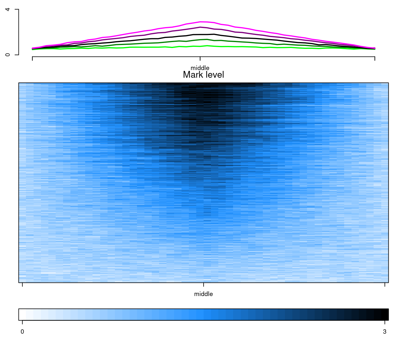
par(old_par)
layout(1)

Session Info

sessionInfo()
#> R version 4.1.1 (2021-08-10)
#> Platform: x86_64-pc-linux-gnu (64-bit)
#> Running under: Ubuntu 20.04.3 LTS
#> 
#> Matrix products: default
#> BLAS:   /usr/lib/x86_64-linux-gnu/blas/libblas.so.3.9.0
#> LAPACK: /usr/lib/x86_64-linux-gnu/lapack/liblapack.so.3.9.0
#> 
#> locale:
#>  [1] LC_CTYPE=fr_FR.UTF-8       LC_NUMERIC=C              
#>  [3] LC_TIME=fr_FR.UTF-8        LC_COLLATE=fr_FR.UTF-8    
#>  [5] LC_MONETARY=fr_FR.UTF-8    LC_MESSAGES=fr_FR.UTF-8   
#>  [7] LC_PAPER=fr_FR.UTF-8       LC_NAME=C                 
#>  [9] LC_ADDRESS=C               LC_TELEPHONE=C            
#> [11] LC_MEASUREMENT=fr_FR.UTF-8 LC_IDENTIFICATION=C       
#> 
#> attached base packages:
#>  [1] grid      parallel  stats4    stats     graphics  grDevices utils    
#>  [8] datasets  methods   base     
#> 
#> other attached packages:
#> [1] EnrichedHeatmap_1.22.0 ComplexHeatmap_2.9.4   ggplot2_3.3.5         
#> [4] epistack_0.99.0        GenomicRanges_1.44.0   GenomeInfoDb_1.28.1   
#> [7] IRanges_2.26.0         S4Vectors_0.30.0       BiocGenerics_0.38.0   
#> 
#> loaded via a namespace (and not attached):
#>  [1] locfit_1.5-9.4         Rcpp_1.0.7             lattice_0.20-45       
#>  [4] circlize_0.4.13        png_0.1-7              assertthat_0.2.1      
#>  [7] digest_0.6.28          foreach_1.5.1          utf8_1.2.2            
#> [10] R6_2.5.1               evaluate_0.14          highr_0.9             
#> [13] blogdown_1.5           pillar_1.6.2           GlobalOptions_0.1.2   
#> [16] zlibbioc_1.38.0        rlang_0.4.11           jquerylib_0.1.4       
#> [19] magick_2.7.3           GetoptLong_1.0.5       rmarkdown_2.11        
#> [22] labeling_0.4.2         stringr_1.4.0          RCurl_1.98-1.3        
#> [25] munsell_0.5.0          compiler_4.1.1         xfun_0.26             
#> [28] pkgconfig_2.0.3        shape_1.4.6            htmltools_0.5.2       
#> [31] tidyselect_1.1.1       tibble_3.1.5           GenomeInfoDbData_1.2.6
#> [34] bookdown_0.22          codetools_0.2-18       matrixStats_0.60.1    
#> [37] fansi_0.5.0            viridisLite_0.4.0      crayon_1.4.1          
#> [40] dplyr_1.0.7            withr_2.4.2            bitops_1.0-7          
#> [43] jsonlite_1.7.2         gtable_0.3.0           lifecycle_1.0.1       
#> [46] DBI_1.1.1              magrittr_2.0.1         scales_1.1.1          
#> [49] stringi_1.7.5          farver_2.1.0           XVector_0.32.0        
#> [52] doParallel_1.0.16      bslib_0.3.1            ellipsis_0.3.2        
#> [55] generics_0.1.0         vctrs_0.3.8            RColorBrewer_1.1-2    
#> [58] rjson_0.2.20           iterators_1.0.13       tools_4.1.1           
#> [61] glue_1.4.2             purrr_0.3.4            plotrix_3.8-1         
#> [64] fastmap_1.1.0          yaml_2.2.1             clue_0.3-59           
#> [67] colorspace_2.0-2       cluster_2.1.2          knitr_1.36            
#> [70] sass_0.4.0